Support Vector Machines (SVMs) | Complete guide support vector machine algorithm - Python Ocean

SVMs are a type of supervised learning algorithm that can be used for classification and regression tasks. The basic idea behind SVMs is to find a linear boundary (or hyperplane) that separates the data points of different classes in a high-dimensional feature space. The boundary is chosen so that it maximizes the margin, which is the distance between the boundary and the closest data points of each class.

SVMs can handle non-linearly separable data by transforming the data into a higher-dimensional space, where a linear boundary can be found. This is done by using a technique called the kernel trick, which applies a non-linear function to the data before it is transformed into a higher-dimensional space.

The algorithm can be broken down into the following steps:

1. Select a kernel function and its parameters
2. Obtain a set of labeled training data
3. Transform the training data into a higher-dimensional space using the kernel function
4. Find the optimal linear boundary that separates the classes in this higher-dimensional space
5. Use the boundary to classify new data points.

SVMs are widely used in various applications such as text and hypertext categorization, image classification, bioinformatics, and face detection.

It's important to note that while SVMs are powerful algorithms, they can be sensitive to the choice of kernel and the scale of the input data. It's also computationally intensive for large datasets.

Understanding kernels in SVM

In Support Vector Machines (SVMs), a kernel is a function that transforms the input data into a higher-dimensional space, where a linear boundary can be found. The kernel trick is used to avoid the computational cost of explicitly calculating the transformation, which can be very expensive for large datasets.

The kernel trick works by replacing the dot product of the input data with the kernel function. This allows SVMs to find a linear boundary in a high-dimensional feature space without the need to explicitly calculate the transformation of the input data.

There are several commonly used kernel functions in SVMs, including:

• Linear kernel: k(x,y) = xT y
• Polynomial kernel: k(x,y) = (xT y + c)^d
• Radial basis function (RBF) kernel: k(x,y) = exp(-γ||x-y||^2)
• Sigmoid kernel: k(x,y) = tanh(γxT y + c)

Each kernel function has its own set of parameters that can be tuned to optimize the performance of the SVM. The choice of kernel function depends on the characteristics of the data and the problem you are trying to solve.

Linear kernel is the simplest one and it is good for linearly separable data, polynomial and RBF kernel are good for non-linearly separable data and sigmoid kernel is good for binary classification.

It's important to note that while kernel functions can improve the performance of SVMs on non-linearly separable data, they can also lead to overfitting, so it's important to use cross-validation to select the best kernel and its parameters for a given dataset.

Implementation

Lets do classification of iris dataset, for simplicity, lets go with first two features, sepal length & sepal width as input label. (Code from scratch is also provided at end of blog)

First Lets import essential libraries

# loading essential modules
from sklearn import datasets
from sklearn import svm
from sklearn.model_selection import train_test_split
import matplotlib.pyplot as plt
from sklearn.metrics import accuracy_score, precision_score, recall_score, f1_score

Then split dataset into training and testing samples

#loading iris dataset
iris = datasets.load_iris()
X = iris.data[:,:2]
y = iris.target
# splitting data into train test samples
X_train, X_test, y_train, y_test = train_test_split(X, y, test_size=0.4, random_state=0)

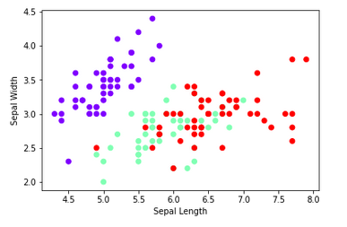
Let's visualize our dataset

plt.scatter(X[:, 0], X[:, 1], c=y, cmap='rainbow')
plt.xlabel('Sepal Length')
plt.ylabel('Sepal Width')
plt.show()

Lets create an instance of the SVM classifier, specifying the kernel type and other relevant parameters

#creating an instance of the SVM classifier 
clf = svm.SVC(kernel='linear', C=1, random_state=0)
# fitting data
clf.fit(X_train, y_train)
y_pred = clf.predict(X_test)

Now Let's evaluate the classifier's performance using various metrics such as accuracy, precision, recall, and F1-score.

print("Accuracy:", accuracy_score(y_test, y_pred))
print("Precision:", precision_score(y_test, y_pred, average='weighted'))
print("Recall:", recall_score(y_test, y_pred, average='weighted'))
print("F1-score:", f1_score(y_test, y_pred, average='weighted'))

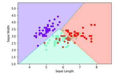
Lets evaluate results by plotting end results

# Plot the decision boundary
import numpy as np
plt.scatter(X[:, 0], X[:, 1], c=y, cmap='rainbow')
plt.xlabel('Sepal Length')
plt.ylabel('Sepal Width')

# Create a mesh grid for plotting
x_min, x_max = X[:, 0].min() - 1, X[:, 0].max() + 1
y_min, y_max = X[:, 1].min() - 1, X[:, 1].max() + 1
xx, yy = np.meshgrid(np.linspace(x_min, x_max, 100),
                     np.linspace(y_min, y_max, 100))

# Plot the decision boundary
Z = clf.predict(np.c_[xx.ravel(), yy.ravel()])
Z = Z.reshape(xx.shape)
plt.contourf(xx, yy, Z, cmap='rainbow', alpha=0.3)
plt.show()

Maths Behind SVM and Implementation from scratch

To dive a little deeper into the math behind support vector machines (SVMs), let's start by considering a binary classification problem, where the goal is to separate two classes of data using a hyperplane. The hyperplane is defined by a set of weights, w, and an offset term, b.

The equation for the hyperplane is:

w^T x + b = 0

where x is a data point, and w^T is the transpose of w. The goal of the SVM algorithm is to find the values of w and b that maximize the margin, which is the distance between the hyperplane and the closest data points from each class. These closest points are called the support vectors.

A simple way to find the hyperplane is to use the perceptron algorithm, which is a linear classifier that tries to find the weights that minimize the classification error. However, this approach does not take into account the margin, and it is sensitive to the presence of outliers.

To find the hyperplane that maximizes the margin, we can cast the problem as a quadratic optimization problem. Given a set of training data, we need to find the values of w and b that minimize:

1/2 * ||w||^2

subject to the constraints:

y_i(w^T x_i + b) >= 1 for i = 1, 2, ..., n

where x_i is a data point, y_i is the corresponding label (1 or -1), n is the number of data points, and ||w|| is the norm of w.

The optimization problem is to minimize the L2-norm of the weight vector w and this is equivalent to maximizing the margin.

This optimization problem can be solved using quadratic programming (QP) methods, but it becomes computationally expensive for large datasets.

To handle non-linearity in the data, we can use a kernel trick where we map the input data into a higher dimensional space using a kernel function. This allows us to use the same optimization algorithm as before, but with the kernel function replacing the inner product of the input data.

Some examples of kernel functions are the polynomial kernel, k(x,x') = (x^T x')^d, and the radial basis function (RBF) kernel,

k(x,x') = exp(-||x-x'||^2 / 2*sigma^2).

These kernel functions are used to calculate dot product between two input vectors in higher dimension space.

Once the hyperplane is found, the support vectors are the points closest to the hyperplane, and the distance between the hyperplane and the closest points is known as the margin. The goal of the SVM is to find the hyperplane with the maximum margin.

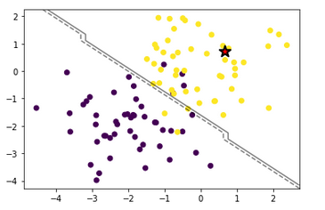
Here is implementation from scratch with description:

import numpy as np
import matplotlib.pyplot as plt

class SVM:

    def __init__(self, C=1):
        self.C = C
        self.w = None
        self.b = None
    
    def fit(self, X, y, learning_rate=0.001, epochs=100):
        n_samples, n_features = X.shape
        w = np.zeros(n_features)
        b = 0

        for epoch in range(epochs):
            for i, x in enumerate(X):
                if (y[i] * (np.dot(w, x) + b)) < 1:
                    w = w + learning_rate * (self.C * y[i] * x - 2 * (1 / epochs) * w)
                    b = b + learning_rate * (self.C * y[i] - 2 * (1 / epochs) * b)
                else:
                    w = w + learning_rate * (-2 * (1 / epochs) * w)
                    b = b + learning_rate * (-2 * (1 / epochs) * b)
        
        self.w = w
        self.b = b
        
    def predict(self, X):
        return np.sign(np.dot(X, self.w) + self.b)

def generate_data():
    np.random.seed(0)
    X = np.random.randn(100, 2)
    y = np.ones(100)
    X[:50, :] = X[:50, :] - 2 * np.ones((50, 2))
    y[:50] = -1
    return X, y

def visualize_results(X, y, clf):
    plt.scatter(X[:, 0], X[:, 1], c=y)
    ax = plt.gca()
    xlim = ax.get_xlim()
    ylim = ax.get_ylim()
    xx = np.linspace(xlim[0], xlim[1], 30)
    yy = np.linspace(ylim[0], ylim[1], 30)
    YY, XX = np.meshgrid(yy, xx)
    xy = np.vstack([XX.ravel(), YY.ravel()]).T
    Z = clf.predict(xy).reshape(XX.shape)
    ax.contour(XX, YY, Z, colors='k', levels=[-1, 0, 1], alpha=0.5,
               linestyles=['--', '-', '--'])
    ax.scatter(clf.w[0], clf.w[1], s=200, marker='*', lw=2, c='red', edgecolor='k')
    plt.show()

if __name__ == '__main__':
    X, y = generate_data()
    clf = SVM(C=1)
    clf.fit(X, y)
    visualize_results(X, y, clf)